acknowledgement

Born, raised, educated, trained and work on lands of the Neutral, Anishinaabeg, Haudenosaunee, Mississaugas, and Secwépemc. Benefits and achievements from time spent on treaty lands including Haldimand Tract of the Six Nations, the Dish with One Spoon Covenant, and unceded lands of Tk’emlúps.

juliatimings

This documents the timings of a simple newton method in R, C (technically cpp but it’s all just C code), and julia.

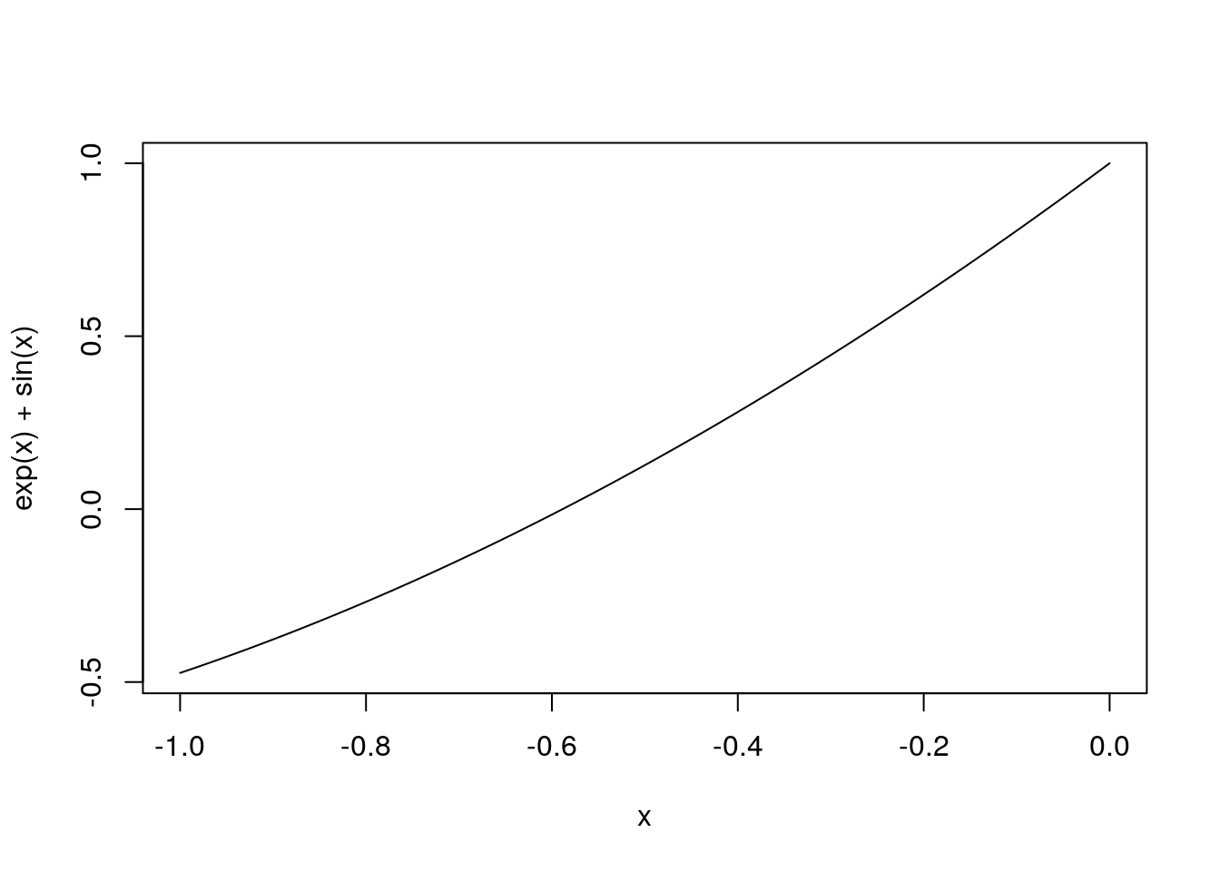
The function is $f_0(x)=e^x+\sin(x)$ so the newton update would be $$x\leftarrow x-\frac{f_0(x)}{f_1(x)}=x-\frac{e^x+sin(x)}{e^x+cos(x)}$$

applied repeatedly. A graph of the curve is shown below. It’s already fairly linear so the function will hit the root very quickly but that’s ok.

curve(exp(x)+sin(x),-1,0)

We'll run the code a fixed number of iterations. I don't know if hitting 0 in the numerator does any short-cutting in any language but thats ok for now.

f0(x)=exp(x)+sin(x)

## f0 (generic function with 1 method)

f1(x)=exp(x)+cos(x)

## f1 (generic function with 1 method)

update(x)=x-f0(x)/f1(x)

## update (generic function with 1 method)

function getroot_julia()
  x=0.0
    for i in 1:50000
        x=update(x)
    end
    return x
end

## getroot_julia (generic function with 1 method)



using BenchmarkTools
timing_julia = @benchmark getroot_julia() samples=5 evals=5

## BenchmarkTools.Trial: 
##   memory estimate:  0 bytes
##   allocs estimate:  0
##   --------------
##   minimum time:     1.020 ms (0.00% GC)
##   median time:      1.028 ms (0.00% GC)
##   mean time:        1.030 ms (0.00% GC)
##   maximum time:     1.044 ms (0.00% GC)
##   --------------
##   samples:          5
##   evals/sample:     5

print(timing_julia)

## Trial(1.020 ms)

getroot_r=function(){
  x=0.0
  ee=0
  for (i in 1:50000){
    ee=exp(x)
    x=x-(ee+sin(x))/(ee+cos(x))
  }
  return (x);
}

the c code

#include <Rcpp.h>
using namespace Rcpp;

//[[Rcpp::export]]
double getroot_cpp() {
  double x=0.0;
  double ee=0.0;
  for(int i=0;i<50000;i++){
    ee=exp(x);
    x=x-(ee+sin(x))/(ee+cos(x));
  }
  return (x);
}

library(JuliaCall)
julia_command("f0(x)=exp(x)+sin(x)")

## Julia version 1.6.0 at location /opt/julia-1.6.0/bin will be used.

## Loading setup script for JuliaCall...

## Finish loading setup script for JuliaCall.

## f0 (generic function with 1 method)

julia_command("f1(x)=exp(x)+cos(x)")

## f1 (generic function with 1 method)

julia_command("update(x)=x-f0(x)/f1(x)")

## update (generic function with 1 method)

julia_command("function getroot_julia()
    x=0.0
    for i in 1:50000
        x=update(x)
    end
    return x
end")

## getroot_julia (generic function with 1 method)

Results

Now that all the functions are created and available, they’re assessed in R. Each runs the same number of iterations with the same initial guess. Each language’s implementation is run a few times times.

library(microbenchmark)
results = microbenchmark(getroot_r(),getroot_cpp(),julia_eval("getroot_julia()"),times=5)

languages = c("R","cpp","julia")
boxplot(results,names=languages)

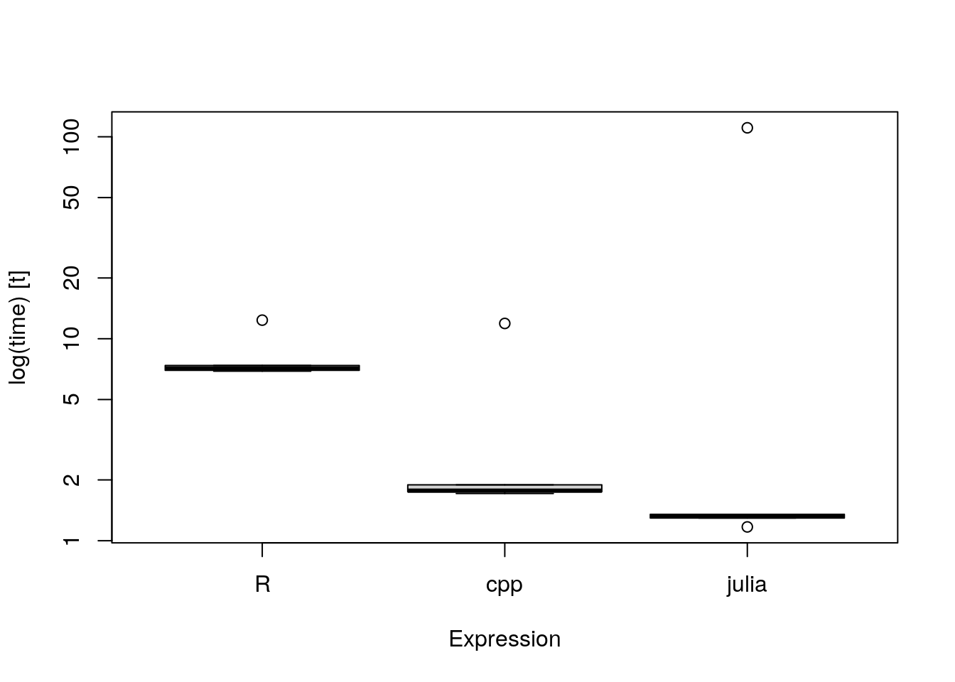
print(results)

## Unit: milliseconds
##                           expr      min       lq      mean   median       uq
##                    getroot_r() 6.909239 6.978445  8.151796 7.135719 7.372746
##                  getroot_cpp() 1.712824 1.747627  3.805588 1.769192 1.890966
##  julia_eval("getroot_julia()") 1.170483 1.295313 23.182798 1.325362 1.350895
##        max neval
##   12.36283     5
##   11.90733     5
##  110.77194     5

medians = summary(results)[,"median"]
names(medians)=languages

#speeds relative to r
medians/max(medians)

##         R       cpp     julia 
## 1.0000000 0.2479347 0.1857363

#speeds relative to julia
medians/min(medians)

##        R      cpp    julia 
## 5.383977 1.334875 1.000000

Hello R Markdown

R Markdown

This is an R Markdown document. Markdown is a simple formatting syntax for authoring HTML, PDF, and MS Word documents. For more details on using R Markdown see http://rmarkdown.rstudio.com.

You can embed an R code chunk like this:

summary(cars)
##      speed           dist       
##  Min.   : 4.0   Min.   :  2.00  
##  1st Qu.:12.0   1st Qu.: 26.00  
##  Median :15.0   Median : 36.00  
##  Mean   :15.4   Mean   : 42.98  
##  3rd Qu.:19.0   3rd Qu.: 56.00  
##  Max.   :25.0   Max.   :120.00
fit <- lm(dist ~ speed, data = cars)
fit
## 
## Call:
## lm(formula = dist ~ speed, data = cars)
## 
## Coefficients:
## (Intercept)        speed  
##     -17.579        3.932

Including Plots

You can also embed plots. See Figure 1 for example:

par(mar = c(0, 1, 0, 1))
pie(
  c(280, 60, 20),
  c('Sky', 'Sunny side of pyramid', 'Shady side of pyramid'),
  col = c('#0292D8', '#F7EA39', '#C4B632'),
  init.angle = -50, border = NA
)

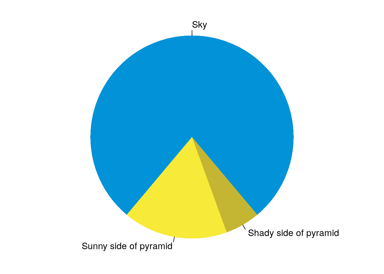
Figure 1: A fancy pie chart.